Vinamax

Fourth example: Electron Paramagnetic Resonance

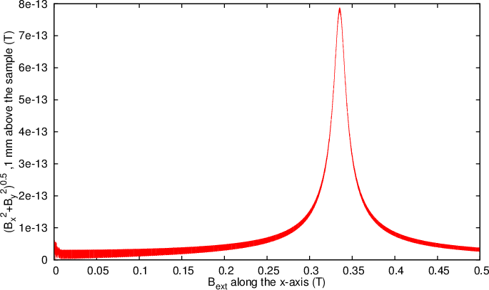
This example illustrates how vinamax can be used to do EPR (electron paramagnetic resonance) simulations. Wikipedia states : "For the microwave frequency of 9388.2 MHz, the predicted resonance position is a magnetic field of about B = 0.3350 tesla". In this example this we will verify if this result can be found with vinamax.

package main

import (
"math"
. "github.com/JLeliaert/vinamax"
)

func main() {

//Defines the world at location 0,0,0 and with a side of 1e-8 m
World(0,0,0,1e-8)
//Adds a single particle in the origin
Addsingleparticle(0,0,0)

//the particle has radius 500 nm
Particle_radius(500e-9)

// An external field is applied that is a sine along the x-axis with amplitude 5 mT and frequency 9388?2 MHz
// Along the z-axis an external field is applied with
B_ext = func(t float64) (float64, float64, float64) { return 0.0005*math.Sin(2*math.Pi*t*9388.2e6), 0., t*0.5/1e-5 }

//Don't calculate demag
Demag=false

//Set saturation magnetisation to 400 000
Msat (400000)

//timestep : 200fs
Dt = 2e-13
//initialise time at zero
T = 0.
//temperature=0
Temp = 0.
//Gilbert damping constant=0.02
Alpha = 0.02
//anisotropy constant=0
Ku1 = 0

//anisotropy axis along the y-direction
Anisotropy_axis(0, 0, 1)

//initialise the magnetisation along the z direction
M_uniform(0,0,1)
//Add the external field to the outputtable
Tableadd("B_ext")
//Probe the demagnetising field at a location of 1 mm above the center of the sample
Tableadd_b_at_location(0.,0.,1e-3)

//write output every nanosecond
Output(1e-9)

//Ask for a suggested timestep
Suggesttimestep()

//run for 1 microsecond
//Here we show how you can define your own variables and use them in the inputfiles:
//A variable "a" is defined which is equal to 1e-5
a:=1.e-5
//and then it is used to tell the simulation how long to run
Run(a)
}

The results of the simulation are visualised below. In the figure it can indeed be seen that there is a resonance peak at the applied field of 0.3350 Tesla.

Suggested Timestep

In the inputfile the function "Suggesttimestep()" is called At the end of the simulation this function returns an estimate of the timestep that would be ideal to perform this simulation. Smaller timesteps would result in larger simulation times, but not in a more accurate result, while larger timesteps would result into less accurate results.

In this example

A good timestep would be:  3.9062789055674464e-13