Vinamax

Fifth example: Profiling

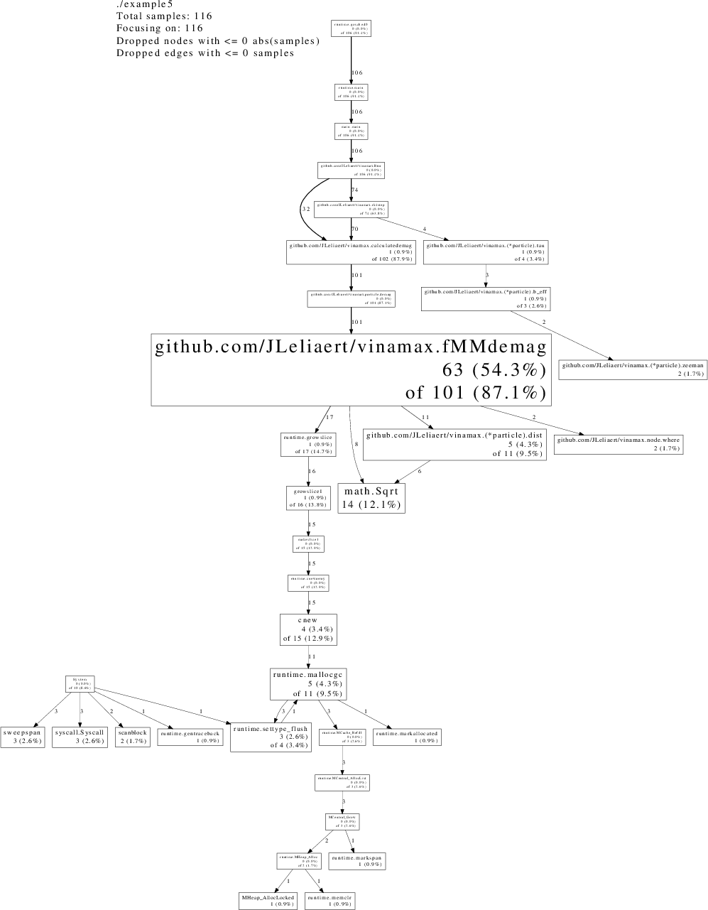
This example shows a how a profile can be made with gotool s. The profile of example3 is made as an illustration.

package main

import (
        . "github.com/JLeliaert/vinamax"
        "flag"
        "log"
        "math"
        "os"
        "runtime/pprof"
)

var cpuprofile = flag.String("cpuprofile", "", "write cpu profile to file")

func main() {

        flag.Parse()
        if *cpuprofile != "" {
                f, err := os.Create(*cpuprofile)
                if err != nil {
                        log.Fatal(err)
                }           
                pprof.StartCPUProfile(f)
                defer pprof.StopCPUProfile()
        }           

        //Defines the world at location 0,0,0 and with a side of 5e-7 m     
        World(0,0,0,5e-7)

        //Adds a cube to the word with side 5e-7 m
        test := Cube{S:5e-7} 
        //Adds 20 particles to the cube
        test.Addparticles(20)

        //the particle have radius 16 nm
        Particle_radius(16e-9)

        //external field along the x direction of 1mT
        //B_ext can be an arbitrary function of time

        B_ext = func(t float64) (float64, float64, float64) { return 0.001,0.,0.0}

        //Calculate the demagnetsing field using the fast multipole method
        //the tresholdbeta= 0.3 is a good compromise between speed and accuracy
        FMM=true
        Thresholdbeta=0.3
        Demag=true

        //saturation magnetisation
        Msat (860e3)

        //timestep : 3e-13s
        Dt = 3e-13
        //initialise time at zero
        T = 0.
        //temperature=0
        Temp = 0.00 K
        //Gilbert damping constant=0.1
        Alpha = 0.1
        //anisotropy constant=0
        Ku1 = 0 J/m**3
        //anisotropy axis along the z-direction
        Anisotropy_axis(0, 0, 1)

        //initialise the magnetisation along the y direction
        M_uniform(0,1,0)
        //Adds the external field to the outputtable
        Tableadd("B_ext")

        //write output every 2e-12s
        Output(2e-12)

        //saves the geometry of the simulation
        Save("geometry")

        //calculates the tree for the FMM demag
        Maketree()


        //run for 1 ns
        Run(1.e-9)
        //saves the magnetisation of particles in the simulation
        Save("m")
}

The bash script below shows how the actual profile can be generatied

#!/bin/bash
go build example5.go
./example5 -cpuprofile=run.prof
go tool pprof --pdf ./example5 run.prof >profile.pdf