Vinamax

Sixth example: Relaxation

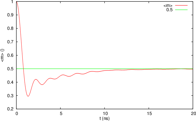
The diameter of the particles can be given a lognormal distribution. This example shows how an ensemble of 20000 particles which are initially magnetised in the z-direction relaxes towards a random (per particle) anisotropy direction.

package main

import (
. "github.com/JLeliaert/vinamax"
)

func main() {

//Defines the world at location 0,0,0 and with a side of 2e-5 m
World(0,0,0,2e-5)

//Adds a cube to the word with side 2e-5 m
test := Cube{S:2e-5}

//Adds 20000 particles to the cube
test.Addparticles(20000)

//the particles have a lognormal distribution of diameters
//with mean 20 nm and stdev 1 nm of the log of the diameters
Lognormal_diameter(20e-9, 1e-9)

//Don't calculate the demagnetsing field
Demag=false

//saturation magnetisation 860 000 A/m
Msat (860e3)

//timestep : 2ps
Dt = 2e-12
//initialise time at zero
T = 0.
//temperature=0
Temp = 0.0
//Gilbert damping constant=0.05
Alpha = 0.05
//anisotropy constant=10 000 J/m**3
Ku1 = 10000

//anisotropy axis is random for every particle
Anisotropy_random()

//initialise the magnetisation along the z direction
M_uniform(0,0,1)

//write output every 4e-12s
Output(4e-12)
//Save the magnetisation at the start of the simulation (to see the diameters)
Save("m")

//run for 20 ns
Run(20.e-9)
}

The results of the simulation are visualised below. The particles are initialised with their magnetisation parallel to the z-axis. They have a random anisotropy axis, so they relax towards this axis (above the horizontal plane) The average magnetisation thus relaxes towards 2/Pi. This value is the mean of cos(x) between O and pi.

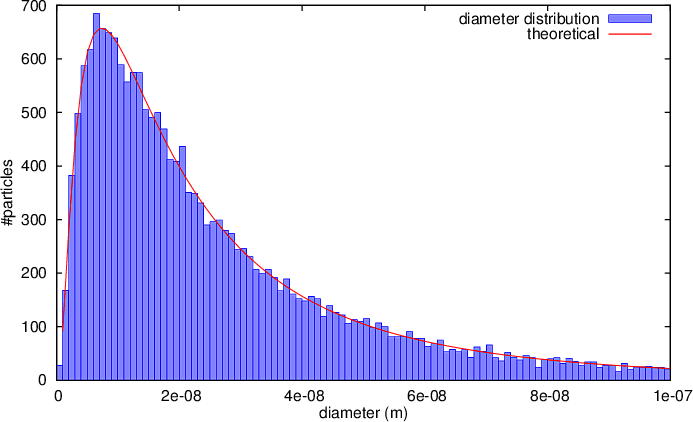
The diameters of the particles was taken from a lognormal distribution, to prove that this is implemented correctly, the distribution of the particles is shown, together with the theoretical curve they are supposed to follow.